
Weekly Bond Yield Forecast and FX Forecast, May 31, 2024: 10-Year Bond Yield Range in 10 Years (EUR:USD)

Instamatics
Diary
This simulation was conducted in conjunction with a simulation of US Treasury yields in a way that reflects the correlation between the 12 factors that drive yields in each country. For more information about the accompanying US Treasury simulation, please contact the author. both of them Simulating US Bond and Treasury yields affects foreign exchange rates, resulting in the following distribution of the EUR/USD exchange rate after one year:
SAS Institute Company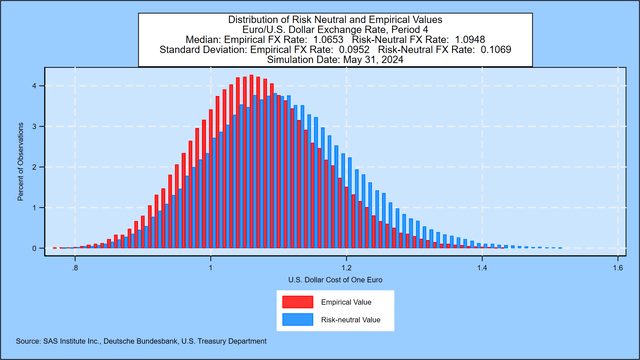
Here are the prices for short and long options to buy EUR/USD with a strike price of 1.07 for quarterly maturities up to 30 years:
SAS Institute Company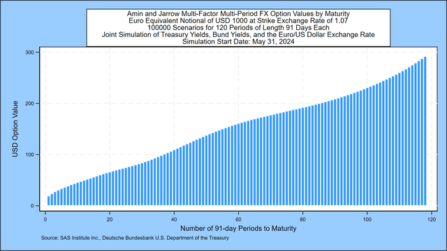
Simulating Bond returns for this week
As explained in Professor Robert Jarrow’s book, mentioned below, forward prices contain a risk premium that exceeds the market’s expectation of the 3-month forward price. We document size The risk premium in the chart below, which shows the zero coupon yield curve indicated by current German Bund rates compared to the compound annual return on 3-month Treasury bills that market participants would expect based on the daily movement of government bond yields in 14 countries. Since 1962. The risk premium, which is the reward for long-term investing, is moderately positive and remains so over the full maturity period up to 30 years. The chart also shows a steady downward shift in returns in the first seven years, as shown below, followed by a gradual rise.
SAS Institute Company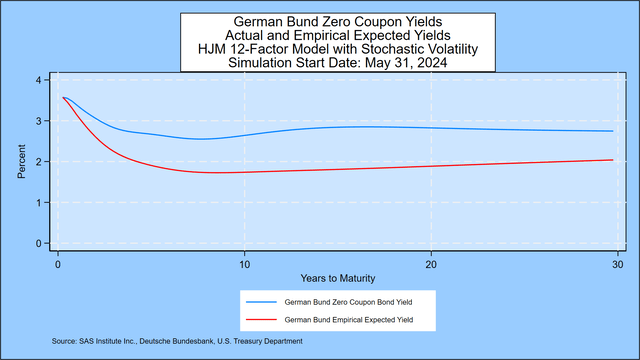
For more on this topic, see the analysis of government bond yields in 14 countries through April 30, 2024, provided in the Appendix.
Inverted yields, negative interest rates and the prospects for German bonds for the next ten years
In this week’s Eurozone forecast, the focus is on three elements of interest rate behavior: the future probability of an inverted yield curve predicting a recession, the probability of negative interest rates, and the probability distribution of German bond yields over the next decade.
We start from the closing German Bund yield curve published daily by the German central bank Deutsche Bundesbank and other information sources. Using a maximum forward rate approach, Friday’s implied forward rate curve shows one-month rates at an initial peak of 3.58%, compared to 3.60% last week. As maturities lengthen, there is some volatility until interest rates peak again at 3.34%, compared to 3.23% last week, and then fall to a lower level of 2.61%, compared to 2.53% last week, at the end of the 30-year horizon. . .
SAS Institute Company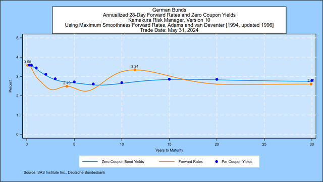
Using the methodology described in the Appendix, we simulated 100,000 thirty-year future paths of the German Bund yield curve. The following three sections summarize our conclusions from those simulations.
Inverted Bond Yields: Inverted now, 69.5% probability by November 29, 2024
Many economists have concluded that a sloping yield curve is an important indicator of a future recession. A recent example of this is this paper by Alex Domash and Lawrence Summers.
We measure the probability that the 10-year nominal coupon bond yield will be less than the 2-year nominal coupon bond yield for each scenario in each of the first 80 quarterly periods in the simulation. (1) The following chart indicates the probability that the inverse return will peak at 69.5% in the 91-day quarterly period ending November 29, 2024, compared to 74.6% last week.
SAS Institute Company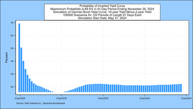
Negative 3-month returns: 21.2% probability by January 23, 2054
The following chart describes the probability of negative interest rates for 3-month bills for all but the first three months of the next three contracts. The probability of negative interest rates starts near zero but peaks at 21.2%, compared to 21.2% last week, for the period ending January 23, 2054.
SAS Institute Company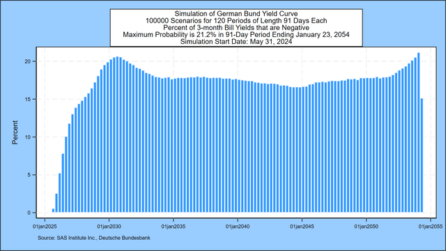
Calculate default risk from interest rate maturity mismatch
In light of the failure of US Silicon Valley Bank due to interest rate risks on March 10, 2023, we have added a table that applies equally to banks and institutional investors and a mismatch for retail investors from long-term buy-in. German short-term borrowed money bonds. We assume that the only asset is the 10-year German Bund purchased at time zero with a nominal value of €100. We analyze default risk for four different ratios of the initial market value of stocks to the market value of assets: 5%, 10%, 15%, and 20%. For the banking example, we assume that the only class of liabilities are deposits that can be withdrawn at nominal value at any time. In the case of institutional and retail investors, we assume that the commitment is essentially borrowing on margin/repurchase agreement with the possibility of a margin call. For all investors, the liability amount (95, 90, 85 or 80) represents the “strike price” on the call option held by the liability holders. Failure occurs via margin call, bank withdrawal, or regulatory takeover (in the case of banking) when the value of assets falls below the value of liabilities.
The chart below shows the cumulative 10-year probabilities of failure for each of the four possible capital ratios when the asset has a 10-year maturity. For the 5% case, the probability of default is 44.05%, a change from 43.64% last week.
SAS Institute Company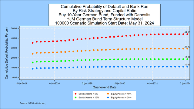
This hypothetical probability analysis is updated weekly based on the German Bund yield simulation described in the next section. The calculation process is the same for any asset portfolio that includes credit risk.
Probabilities of German bond returns for the next ten years
In this section, the focus turns to the next decade. This week’s simulation shows that the most likely range for the 3-month bond yield in the bond market in ten years is 0% to 1%, unchanged from last week. There is a 25.61% probability that the 3-month yield will fall into this range, which is a change from 25.87% one week ago. Note the downward shift in the second and third semiannual periods. For the 10-year German Bund yield, the most likely range is 1% to 2%, also unchanged from last week. The probability of being in this range is 21.86%, compared to 22.02% one week ago.
In a recent post on Seeking Alpha, we pointed out that predicting “heads” or “heads” on a coin toss ignores important information. What an experienced bettor needs to know is that on average for a fair coin, the probability of coming heads is 50%. Predicting that the next side of the coin will be “heads” is worth nothing to investors, because the outcome is completely random.
The same applies to interest rates.
In this section, we present the detailed probability distribution of both the 3-month bill rate and the 10-year bond yield after 10 years using semiannual time steps(2). We give the probability of locating rates at each time step in “rate clusters” as 1 percent. 3-month bond yield forecasts are shown in this chart:
SAS Institute Company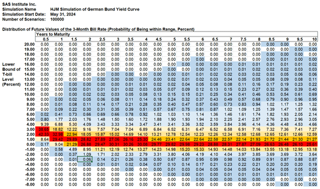
Invoice return data for 3 months:
SASDEU3m20240531.xlsx
Shown in Column 4: The probability that the 3-month billing return will be between 1% and 2% in 2 years. The probability that the 3-month return will be negative (as it often was in Europe and Japan) in 2 years is 8.95% plus 1.09% plus 0.06% plus 0.00% = 10.10% (the difference is due to rounding). Blue shaded cells represent positive probabilities of occurrence, but the probability has been rounded to the nearest 0.01%. The shading system works as follows:
- Dark blue: Probability is greater than 0% but less than 1%
- Light blue: Probability is greater than or equal to 1% and less than 5%
- Light yellow: Probability greater than or equal to 5% and 10%
- Medium yellow: Probability greater than or equal to 10% and less than 20%
- Orange: Probability is greater than or equal to 20% and less than 25%
- Red: The probability is greater than 25%.
The chart below shows the same probabilities for the 10-year Bond return derived as part of the same simulation.
SAS Institute Company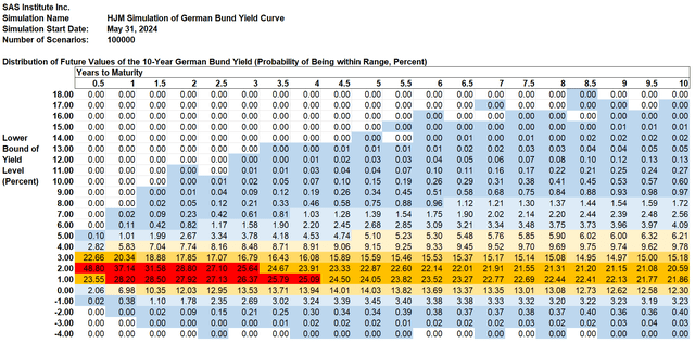
Ten-year German bond yield data:
SASDEU10y20240531.xlsx
Appendix: Bond return simulation methodology
Probabilities are derived using the same methodology that SAS Institute Inc. recommends for its KRIS® and Risk Manager Kamakura® Client. A somewhat technical explanation is given later in the Appendix, but we briefly summarize it first.
Step 1: We take the closing Bond yield curve as a starting point.
Step 2: We use the number of points on the yield curve that best explains historical yield curve shifts. We note in the following chart that the bond returns extend (depending on the price level and maturity) by only 40.69% from the historical experience in 14 countries:
SAS Institute Company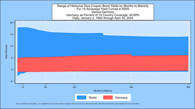
To obtain the highest degree of realism in forward-looking simulations, the use of an international database is essential. Using daily government bond yield data from 14 countries from 1962 through April 30, 2024, we conclude that 12 “factors” drive almost all movements in government bond yields. The countries on which the analysis is based are Australia, Canada, France, Germany, Italy, Japan and New Zealand. Russia, Singapore, Spain, Sweden, Thailand, the United Kingdom, and the United States of America. No data from Russia after January 2022 is included.
Step 3: We measure the volatility of changes in those factors and how volatility changes over the same period.
Step 4: Using those measured volatility, we generate 100,000 random shocks at each time step and infer the resulting yield curve.
Step 5: We “validate” the model to ensure that the simulation prices the initial Bond curve exactly and fits history as closely as possible. The methodology for doing this is described below.
Step 6: We take all 100,000 simulated yield curves and calculate the odds that the yield will fall in each of the 1% “bulldozers” displayed in the chart.
Do nominal yields accurately reflect expected future inflation?
We showed in a recent Seeking Alpha post that investors on average have always done better by buying longer-term bonds than by rolling over short-term US Treasuries. This means that market participants were generally (but not always) accurate in forecasting future inflation and adding a risk premium to those forecasts. This study will be updated using the 14-country dataset in the coming weeks.
Technical details
Daily government bond yields from the above 14 countries constitute the underlying historical data to fit the number of yield curve factors and their volatility. Historical data for the Bund is provided by Deutsche Bundesbank. Using international bond data increases the number of observations to more than 106,000 and provides a more complete range of experience with high rates and negative rates than is provided by the Bond data set alone.
The modeling process was published in an important paper by David Heath, Robert Jarrow and Andrew Morton in 1992:
slandered economy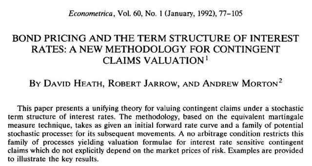
Professor Jarrow’s CV is available here.
The non-arbitrage foreign exchange rate simulation is based on this well-known paper by Amin and Jarrow:
Journal of International Money and Finance
For technically inclined readers, we recommend Professor Jarrow’s book Modeling fixed income securities and interest rate options For those who want to know exactly how the “HJM” model building works.
The number of factors, 12 for the 14-country model, has remained stable since June 30, 2017.
Footnotes:
(1) After the first 20 years of simulation, the 10-year return cannot be derived from the initial 30-year return structure.
(2) The actual simulation uses 91-day time steps and spans a 30-year time horizon.
Editor’s Note: This article discusses one or more small-cap stocks. Please be aware of the risks associated with these stocks.